3Delight 12.0 User's Manual: 7.4 Global Illumination

Short Contents

7.4 Global Illumination

7.4.1 Ambient Occlusion

Ambient occlusion (also known as "geometric exposure") is trivially computed using the occlusion() shadeop (see occlusion shadeop). Objects contributing to occlusion have to be tagged as visible to transmission rays using Attribute "visibility" "transmission" "opaque"(50). occlusion() works by tracing a specified number of rays into the scene or can be provided with a point cloud to compute occlusion using a point-based approximation. The rest of this chapter deals with the ray tracing version of occlusion(), the point-based approach is detailed in Point-Based Occlusion and Color Bleeding.

The number of samples specified as a parameter to occlusion() is a quality vs. speed knob: less samples give fast renders and more noise, more samples yield to longer render times but smoother appearance. 16 to 32 samples is a recommended setting for low quality renders, 128 and more samples are needed for high quality results. It is important to turn RiShadingInterpolation to `smooth'; this increases occlusion() quality, especially on the edges where two different surfaces meet and form a concave feature.

Occlusion can also be returned using the indirectdiffuse() shadeop (see indirectdiffuse shadeop). This is useful when both indirect illumination and ambient occlusion are needed. Note that using indirectdiffuse() to compute occlusion can be much more costly than using occlusion() since it often triggers execution of shader code.

Here is a simple light source shader illustrating the use of occlusion():

**Listing 7.4**: Ambient occlusion using a lightsource shader
light occ_light( float samples = 64; string __category = "occlusion"; float __nonspecular = 1; ) { normal shading_normal = normalize( faceforward(Ns, I) ); illuminate( Ps + shading_normal ) { Cl = 1 - occlusion( Ps, shading_normal, samples ); } }

light occ_light(
  float samples = 64;
  string __category = "occlusion";
  float __nonspecular = 1; )
{
  normal shading_normal = normalize( faceforward(Ns, I) );

  illuminate( Ps + shading_normal )
  {
    Cl = 1 - occlusion( Ps, shading_normal, samples );
  }
}

Listing 7.4: Ambient occlusion using a lightsource shader

7.4.2 Photon Mapping

3DELIGHT supports photon mapping for both caustics and indirect lighting. Photon maps can either be generated in a different pass and stored on disk for re-use, or they can be automatically generated by 3DELIGHT in the main rendering pass and stored in memory only. The next two sections describe the two approaches in detail.

Examples illustrating both methods can be found in `$DELIGHT/examples/photons'.

7.4.2.1 Photon Mapping Concepts

Photon mapping is an elegant technique to render effects such as caustics and multi-bounce global illumination efficiently. The algorithm proceeds by tracing a specified number of "photons" from light sources that are then "bounced" from surface to surface and stored on diffuse surfaces. The stored photons can then be used to compute light irradiance during the main (beauty) pass. The main applications for photon maps are:

Render caustics: To do this, one needs to explicitly call a shadeop to compute irradiance - either by calling photonmap() (see photonmap shadeop) or caustic() (see caustic shadeop).
Render color bleeding using "final gathering": This is trivially achieved by rendering a photonmap and calling indirectdiffuse() which will automatically query photon maps for secondary bounces. More about final gathering in Final Gathering and indirectdiffuse shadeop.
Render fast global illumination previews: This is done by directly using the photon maps to compute irradiance at each sample, without calling indirectdiffuse(). In some cases, this could lead to acceptable results even for final renders.

7.4.2.2 Single Pass Photon Mapping

Here is the list of steps required to enable single pass photon map generation:

Set Option "photon" "emit" to the number of photons to trace.
This indicates to the renderer how many photons are to be traced into the scene. This specifies the total number of photons to trace and not a number for each light: 3DELIGHT will analyze each light such as to trace more photons from brighter lights. The number of photons depends on scene complexity and light placement and can vary between thousands and millions of photons.

Mark primitives visible to photon rays using Attribute "visibility" "photon" [1].
Primitive that are not marked as visible to photons will not be included in the photon tracing process.

Name a global photon map and a caustic photon map using Attribute "photon" "globalmap" and Attribute "photon" "causticmap". These photon map names can then be used to access the photon maps as explained in photonmap shadeop. It is common to set, for the entire scene, only one global map for final gathering and one for caustics but it is perfectly legal to specify one per object or per group of objects.

Select material type for surfaces using Attribute "photon" "shadingmodel".
This will indicate how each surface react to photons. Valid shading models are: `matte', `chrome', `water', `glass' and `transparent'.

Enable photon map generation for desired lights using Attribute "light" "emitphotons" ["on"]. Normally, only spot lights, point lights and directional lights are turned on for photon generation. Light sources that do global illumination work (such as calling occlusion() or indirectdiffuse()) should not cast photons.

In this single pass approach, the total number of bounces -both diffuse and specular- are set using RiOption. For example, to set the total number of bounces to 5, one would write:

Option "photon" "maxdiffusedepth" [5] "maxspeculardepth" [5]

Using the single appoach to photon mapping has some interesting advantages:

Only uses core memory: no data is written to disk if the user doesn't want it.

Simple to use with already established pipelines.

The main drawback being that generated photon maps are not re-usable.

7.4.2.3 Two Pass Photon Mapping

If re-using photon maps is a prerequisite, then the two pass approach can be used to generate the photon maps and save them into files to be used in subsequent renders. This is done much like for the one pass approach but instead of using the Option "photon" "emit" command a special `photon' hider is used:

Hider "photon" "int emit" [100000]

When using this hider, the renderer will not render the scene but instead store all the computed photon maps into files specified by Attribute "photon" "globalmap" and Attribute "photon" "causticmap".Those photon maps can then be read by specifying the same attributes in a normal render (using the `hidden' hider). An example of this approch is found in the `$DELIGHT/examples/photons' directory.
The total number of bounces a photon can travel can be specified on a per-prmitive basis, for example:

Attribute "trace" "maxdiffusedepth" [10] "maxspeculardepth" [5]

7.4.3 Final Gathering

Final gathering is a technique to render global illumination effects (color bleeding) efficiently. In summary, for global illumination rendering using n bounces, the algorithm first proceeds by emitting photons from light sources for the n-1 bounces. Then, the last bounce is simulated by tracing a specified number of rays from surfaces; at each ray-surface intersection the photon map is used to compute the radiance. The main benefit here is that instead of ray tracing the entire n bounces, we only ray trace one bounce and the rest is available through photon maps.
This functionality is readily available using the indirectdiffuse() shadeop (see indirectdiffuse shadeop) which traces a specified number of rays in the scene and collects incoming light. If indirectdiffuse() encounters photon maps on surfaces it will automatically use them and avoid ray tracing, effectively achieving the so called final gathering algorithm.

7.4.4 Image Based Lighting

Integrating synthetic elements into real footage became an important aspect of modern computer imagery. To make the integration of such elements as realistic as possible, it is of prime importance to respect the lighting characteristics of the real environment when rendering the synthetic elements. Lighting characteristics include both the color of the elements as well as the shadows cast by those elements into the real world.

Both imperatives can be achieved by placing lights in the virtual environment that mimic the placement of lights in the real environment. This is usually a tedious task that is also error prone. A more elegant technique relies on photographs of real environments to compute lighting on synthetic elements. Those photographs are usually high dynamic range images taken on set.

Preparing HDR Images

High dynamic ranges images come mostly in two format: light probes or two fisheye images. tdlmake can read both formats and convert them into a cubic environment map usable from shaders. The following example converts a "twofish" environment in EXR format into a cubic environment map usable in 3DELIGHT:

% tdlmake -twofish north.exr south.exr env.tdl

Once the environment is converted into a cubic environment map it can easily be accessed from the shading language.

Using HDR Images

Most people are familiar with the occlusion() shadeop that simulates shadows as cast by a hemispherical light(51). The shadeop proceeds by casting a specified number of rays in the environment and probing for intersections with surrounding geometry. Rays are usually cast uniformly on the hemisphere defined by surface's point and normal. While very useful, this technique is not convincing for non uniformly lit environments. To overcome this problem, 3Delight offers a special gather() construct to extract illumination from an environment map: passing the environment map as a special category to gather() will perform an importance sampling over the environment and provide useful information in the body of the construct:

` environment:direction': The current direction from the environment map. More precisely, the current direction describes the center of a luminous cluster in the environment map. This direction can be used to trace transmission rays to obtain hard shadows.
` environment:solidangle': The solid angle for the current direction. This can be considered as the extent, in space, of the luminous cluster currently considered.
` ray:direction': A random direction inside the luminous cluster described by `environment:direction' and `environment:solidangle'. This can be used to trace transmission rays for to obtain blurry shadows.
` environment:color': The color "coming" from the current environment direction. This is the average color of the luminous cluster.

This is better illustrated in Listing 7.5.

**Listing 7.5**: Using `gather()` to extract lighting information from environment maps.
... /* Assuming that: 'envmap' contains the name of the environment map. 'kocc' containts the shadowing strength. 'envspace' is the space in which the environment is. / string gather_cat = concat("environment:", envmap); color envcolor = 0; vector envdir = 0, raydir = 0; float solidangle = 0; gather( gather_cat, 0, 0, 0, samples, "environment:color", envcolor, "ray:direction", raydir, "environment:direction", envdir, "environment:solidangle", solidangle ) { raydir = vtransform( envspace, "current", raydir ); envdir = vtransform( envspace, "current", envdir ); color trs = transmission( Ps, Ps + raydir maxdist, "bias", bias ); trs = 1 - kocc * (1 - trs); Cl += envcolor * trs; } ...

...
/* Assuming that:
   'envmap' contains the name of the environment map.
   'kocc' containts the shadowing strength. 
   'envspace' is the space in which the environment is. */
string gather_cat = concat("environment:", envmap);
color envcolor = 0;
vector envdir = 0, raydir = 0;
float solidangle = 0;

gather( gather_cat, 0, 0, 0, samples,
    "environment:color", envcolor, "ray:direction", raydir,
    "environment:direction", envdir, "environment:solidangle", solidangle )
{
    raydir = vtransform( envspace, "current", raydir );
    envdir = vtransform( envspace, "current", envdir );

    color trs = transmission( Ps, Ps + raydir * maxdist, "bias", bias );
    trs = 1 - kocc * (1 - trs);
    Cl += envcolor * trs;
}
...

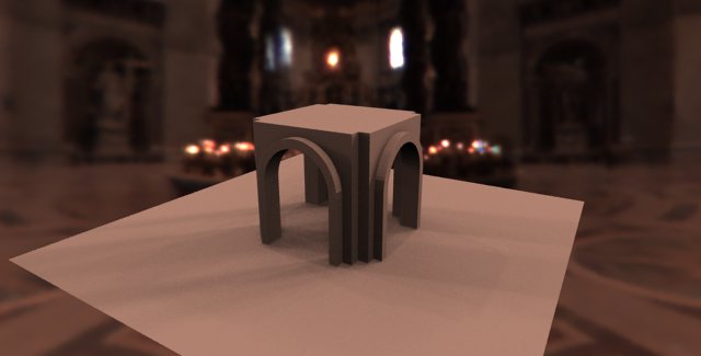
Thanks to the special gather() construct shown in Listing 7.5, it becomes easy to compute image based lighting: transmission rays are traced into the scene to compute the shadowing and the color given by `environment:color' is used directly to compute the environment color. It is recommanded to combined the environment light with surface's BRDF to obtain more realistic results.
If one wants the diffuse environment lighting with no occlusion, it is always possible to call the indirectdiffuse() shadeop (see image based indirectdiffuse). This shadeop provides a simple way to do diffuse image based lighting without texture blurring and a guaranteed smoothly varying irradiance function. indirectdiffuse() efficiently integrates the irradiance coming from distant objects, as described by the provided environment map. No special operations are needed on environment maps: the same environment used for standard reflection mapping can be directly passed as a parameter. One could simply call indirectdiffuse with an environment map and the surface normal to get the diffuse lighting as seen by the [P, N] surface element:

color diffuse_component = indirectdiffuse( envmap, N );

IMPORTANT
Prior 3Delight 7.0, image based lighting was accomplished using occlusion() and indirectdiffuse(). This combination still works as usual but one must be aware that:

occlusion() uses a less than perfect algorithm to detect the luminous clusters in an environment map.
Combining occlusion() and indirectdiffuse() does not yield to "correct" results since the diffuse lighting doesn't take the occlusion into account.

So we strongly recommand using the gather() construct instead of the previous method.

The `envlight2' light shader provided with 3Delight combines both the image based occlusion and indirect diffuse lighting and has been used to produce figure Figure 7.2.

**Figure 7.2**: An image rendered using an HDRI map and the ``envlight2`' shader. There is no "light sources" in the scene: the shadows are cast from bright regions in the environment.

7.4.5 Subsurface Scattering

7.4.5.1 One Pass Point-Based Subsurface Scattering

3Delight features an integrated subsurface light transport algorithm, meaning that subsurface scattering simulations do not need additional passes.
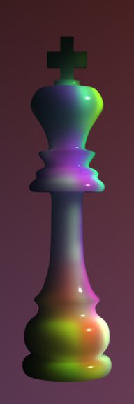
Here is an image created with the example included in the 3Delight distribution (it can be found in `$DELIGHT/examples/subsurface/'):

**Figure 7.3**: Teapot rendered with subsurface scattering enabled.

Running a subsurface simulation is a three step process:

Surfaces defining a closed object are marked as belonging to the same subsurface group.

Subsurface light transport parameters are specified using Attribute "subsurface" on one of the surfaces that is part of the closed object.

Object's surface shader is modified to correctly account for subsurface lighting.

Each operation is further explained below. A functional RIB file can also be found in `$DELIGHT/examples/subsurface'.

Defining a Closed Object

This is done using Attribute "visibility" "subsurface" "groupname"; an example RIB snippet:

AttributeBegin
  Attribute "visibility" "subsurface" "marble"

  ... Object's subsurface light transport parameters go here ...
  ... Object's geometry goes here ...
AttributeEnd

Parts of geometry belonging to the same closed object can be specified anywhere in the RIB, as long as they all belong to the same subsurface group.

Specifying Subsurface Scattering Parameters

Subsurface light transport parameters can be specified in two different ways (see Subsurface Scattering Attributes): the first one is by specifying the reduced scattering coefficient, reduced absorption coefficient and surface's relative index of refraction; the second way is by specifying material's mean free path, diffuse reflectance and index of refraction. All the provided measures should be given in millimeters.

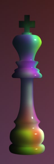
The `shadingrate' attribute has the conventional interpretation and determines how finely irradiance is sampled in the precomputation phase. The default value is 1.0 but larger values should be used for highly scattering materials, greatly improving precomputation speed and memory use as shown in Figure 7.4.


``shadingrate`' = 1.0	= 4.0	= 10.0	= 50.0
Timing = 48 secs	= 40 secs	= 33 secs	= 23 secs
Memory = 43 Megs	= 20 Megs	= 18 Megs	= 16 Megs

Figure 7.4: Highly scattering materials can benefit from higher shading rates. The chess piece is translucent enough to use very high shading rates without affecting quality significantly.

Since geometry is rarely specified in millimeters, a scaling factor, which is applied to the given parameters, can also be provided to 3Delight. For example, specifying a scale of `0.1' means that geometry data is specified in centimeters (objects are ten times bigger). Continuing with the previous RIB snippet:

AttributeBegin
  Attribute "visibility" "subsurface" "marble"

  # marble light scattering parameters
  Attribute "subsurface"
    "color scattering" [2.19 2.62 3.00]
    "color absorption" [0.0021 0.0041 0.0071]
    "refractionindex" 1.5
    "scale" 0.1
    "shadingrate" 1.0

  ... Object's geometry goes here ...
AttributeEnd

Surface properties can be obtained from specialized literature. A reference paper that contains many parameters (such as skin) directly usable in 3Delight:

Henrik Wann Jensen, Stephen R. Marschner, Marc Levoy and Pat Hanrahan. A Practical Model for Subsurface Light Transport. ACM Transactions on Graphics, pp 511-518, August 2001 (Proceedings of SIGGRAPH 2001).

Modifying surface Shaders

3Delight renders subsurface scattering in two passes: it firsts starts a precomputation process on all surfaces belonging to some subsurface group and then starts the normal render. When shaders get executed in the preprocessing stage, rayinfo("type", ...) returns "subsurface". Using this information, a shader can perform conditional execution depending on the context. Here is the standard plastic shader changed as to work with subsurface scattering.

**Listing 7.6**: Simple subsurface shader
surface simple( float Ks = .7, Kd = .6, Ka = .1, roughness = .04 ) { normal Nf = faceforward( normalize(N), I); vector V = normalize(-I); uniform string raytype = "unknown"; rayinfo( "type", raytype ); if( raytype == "subsurface" ) { /* no specular is included in subsurface lighting ... / Ci = Kaamient() + Kddiffuse(Nf); } else { Ci = subsurface(P) + Ks specular(Nf, V, roughness); } }

surface simple( float Ks = .7, Kd = .6, Ka = .1, roughness = .04 )
{
  normal Nf = faceforward( normalize(N), I);
  vector V = normalize(-I);

  uniform string raytype = "unknown";
  rayinfo( "type", raytype );

  if( raytype == "subsurface" )
  {
    /* no specular is included in subsurface lighting ... */
    Ci = Ka*amient() + Kd*diffuse(Nf);
  }
  else
  {
    Ci = subsurface(P) + Ks * specular(Nf, V, roughness);
  }
}

Listing 7.6: Simple subsurface shader

7.4.5.2 Two Pass Point-Based Subsurface Scattering

One disadvantage of using the one-pass method for subsurface scattering is that the pre-computation performed by the renderer is not re-usable from frame to frame. This can be fixed by using a two-pass technique that relies on a point-cloud file to store the intermediate color values.

In the first pass the frame is rendered normally, as a beauty pass, and the result is saved in the `_radiosity' channel of a point-cloud file (if needed, the area of the micro-polygon can be altered by using the `_area' float channel). It is important to correctly set the culling attributes so that hidden surfaces are rendering, as explained in Baking.

In the second pass, the subsurface() shadeop (see subsurface shadeop) is called by specifying the point-cloud file along with the subsurface parameters and is normally blended with the direct illumination as in the one-pass method.

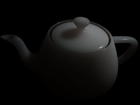
The two pass method is better illustrated using a simple example.

**Listing 7.7**: Example RIB illustrating two-pass subsurface scattering.
Projection "perspective" "fov" [ 35 ] ArchiveBegin "geo" AttributeBegin Translate 0 0 3 Scale 0.25 0.25 0.25 Translate 0 -0.5 0 Rotate -120 1 0 0 Geometry "teapot" AttributeEnd ArchiveEnd LightSource "spotlight" 1 "intensity" [ 120 ] "from" [ 5 3.5 2.5 ] "uniform string shadowmap" "raytrace" "coneangle" [ 2 ] "lightcolor" [ 1 1 1 ] Attribute "visibility" "transmission" "Os" Display "none" "null" "rgb" WorldBegin Surface "simple_bake" "Ks" [ 0.7 ] "roughness" [ 0.02 ] "string bakefile" ["teapot.ptc"] Attribute "cull" "hidden" [0] "backfacing" [0] ReadArchive "geo" WorldEnd Display "teapot_using_ptc.tif" "tiff" "rgb" WorldBegin Surface "simple_using_ptc" "Ks" [ 0.7 ] "roughness" [ 0.02 ] "string bakefile" ["teapot.ptc"] "float scale" [0.05] ReadArchive "geo" WorldEnd

Projection  "perspective" "fov" [ 35 ]

ArchiveBegin "geo"
  AttributeBegin
    Translate  0 0 3 Scale  0.25 0.25 0.25 Translate  0 -0.5 0
	Rotate -120 1 0 0
	Geometry "teapot"
 AttributeEnd
ArchiveEnd

LightSource  "spotlight" 1 
  "intensity" [ 120 ] "from" [ 5 3.5 2.5 ]
  "uniform string shadowmap" "raytrace" 
  "coneangle" [ 2 ] "lightcolor" [ 1 1 1 ]

Attribute  "visibility" "transmission" "Os" 

Display  "none" "null" "rgb"
WorldBegin
  Surface  "simple_bake" 
    "Ks" [ 0.7 ] "roughness" [ 0.02 ] "string bakefile" ["teapot.ptc"]
  Attribute "cull" "hidden" [0] "backfacing" [0]
  ReadArchive "geo"
WorldEnd

Display  "teapot_using_ptc.tif" "tiff" "rgb"
WorldBegin
  Surface "simple_using_ptc"
    "Ks" [ 0.7 ] "roughness" [ 0.02 ] "string bakefile" ["teapot.ptc"] "float scale" [0.05]
  ReadArchive "geo"
WorldEnd

Listing 7.7: Example RIB illustrating two-pass subsurface scattering.

The simple_bake and simple_using_ptc are listed below.

surface simple_bake( float Ks = .7, Kd = .6, Ka = .1, roughness = .04;
  string bakefile = "" )
{
  vector V = normalize(-I);
  Ci = Cs * (Ka*ambient() + Kd*diffuse(normalize(N))) + subsurface(P);
  float A = area(P);
  bake3d( bakefile, "", P, N, "_radiosity", Ci, "_area", A, "interpolate", 1 );
}

surface simple_using_ptc(
  float Ks = .7, Kd = .6, Ka = .1, roughness = .04;
  string bakefile = "";
  color albedo = color(0.830,0.791, 0.753);
  color dmfp = color(8.51, 5.57, 3.95);
  float ior = 1.5, scale = 1.0;  )
{
  normal Nf = faceforward( normalize(N), I);
  vector V = normalize(-I);

  Ci = subsurface(P, Nf,
      "filename", bakefile,
      "diffusemeanfreepath", dmfp, "albedo", albedo,
      "scale", scale, "ior", ior )
    + Ks * specular(Nf, V, roughness);
}

Here is a summary of the major differences with the one-pass techniques:

The subsurface parameters (albedo, diffuse mean free path) are not set by attribute anymore, they are specified to the subsurface() shadeop. The shading rate of the subsurface pass is simply specified using RiShadingRate() in the baking pass.

There is no more subsurface groups: groups are implicitly declared by the geometry rendered and baked in the point-cloud file.

User has the ability to use two different shaders: one for the baking pass and one for the final pass. This is not possible in the one-pass method. In normal situations this isn't desirable though, most of the code line will be shared between the shaders. It is of course necessary not to include the specular component of the illumination model in the pre-pass (this includes reflections and refractions): this is not only inaccurate but also slows down the rendering of the pre-pass.

7.4.5.3 Ray Traced Subsurface Scattering

Ray-traced subsurface scattering has major advantages over the point-based version:

It can compute single scattering effect in addition to multiple scattering.

It doesn't need any pre-computation and works well with IPR.

It is easier to get light blockers inside geometry to have intersting volume shadowing effects.

It has a smaller memory footprint.

It works well on scenes of large scales - a big problem in the point-based version.

Apart from sampling noise at lower sample counts, the overall look is very close to the point-based version and can be used as a drop-in replacement. The semantics are almost exactly the same. Transforming the example in Listing 7.6 is straightforward and is shown in Listing 7.8

**Listing 7.8**: Simple ray traced subsurface shader
surface simple( float Ks = .7, Kd = .6, Ka = .1, roughness = .04 ) { normal Nf = faceforward( normalize(N), I); vector V = normalize(-I); uniform string raytype = "unknown"; rayinfo( "type", raytype ); if( raytype == "subsurface" ) { /* no specular is included in subsurface lighting ... / Ci = Kaamient() + Kddiffuse(Nf); } else { Ci = subsurface(P, Nf, "type", "raytrace", "samples", 64) + Ks specular(Nf, V, roughness); } }

surface simple( float Ks = .7, Kd = .6, Ka = .1, roughness = .04 )
{
  normal Nf = faceforward( normalize(N), I);
  vector V = normalize(-I);

  uniform string raytype = "unknown";
  rayinfo( "type", raytype );

  if( raytype == "subsurface" )
  {
    /* no specular is included in subsurface lighting ... */
    Ci = Ka*amient() + Kd*diffuse(Nf);
  }
  else
  {
    Ci = subsurface(P, Nf, "type", "raytrace", "samples", 64) + Ks * specular(Nf, V, roughness);
  }
}

Listing 7.8: Simple ray traced subsurface shader

Note that we need to pass the surface normal, the type parameter as well as a sample count. Everything else is exactly as in the point-based version.

[ < ]

[ > ]

[ << ]

[ Up ]

[ >> ]